前言
跟着李沐的《动手学深度学习(PyTorch版)》学了一阵子。跟着教程在Kaggle进行一次小演练,源码除了数据预处理部分其他暂时没有改动。
视频链接:15 实战:Kaggle房价预测 + 课程竞赛:加州2020年房价预测【动手学深度学习v2】_哔哩哔哩_bilibili
课程主页:https://courses.d2l.ai/zh-v2/
教材:https://zh-v2.d2l.ai/
题目
House Prices - Advanced Regression Techniques
链接:House Prices - Advanced Regression Techniques | Kaggle
实战
下载和缓存数据集
1
2
3
4
5
6
7
8
9
10
11
12
13
14
15
16
17
18
19
20
21
22
23
24
25
26
27
28
29
30
31
32
33
34
35
36
37
38
39
40
41
42
43
44
45
46
47
48
49
50
| import hashlib
import os
import tarfile
import zipfile
import requests
DATA_HUB = dict()
DATA_URL = 'http://d2l-data.s3-accelerate.amazonaws.com/'
def download(name, cache_dir=os.path.join('..', 'data')):
"""下载一个DATA_HUB中的文件,返回本地文件名"""
assert name in DATA_HUB, f"{name} 不存在于 {DATA_HUB}"
url, sha1_hash = DATA_HUB[name]
os.makedirs(cache_dir, exist_ok=True)
fname = os.path.join(cache_dir, url.split('/')[-1])
if os.path.exists(fname):
sha1 = hashlib.sha1()
with open(fname, 'rb') as f:
while True:
data = f.read(1048576)
if not data:
break
sha1.update(data)
if sha1.hexdigest() == sha1_hash:
return fname
print(f'正在从{url}下载{fname}...')
r = requests.get(url, stream=True, verify=True)
with open(fname, 'wb') as f:
f.write(r.content)
return fname
def download_extract(name, folder=None):
"""下载并解压zip/tar文件"""
fname = download(name)
base_dir = os.path.dirname(fname)
data_dir, ext = os.path.splitext(fname)
if ext == '.zip':
fp = zipfile.ZipFile(fname, 'r')
elif ext in ('.tar', '.gz'):
fp = tarfile.open(fname, 'r')
else:
assert False, '只有zip/tar文件可以被解压缩'
fp.extractall(base_dir)
return os.path.join(base_dir, folder) if folder else data_dir
def download_all():
"""下载DATA_HUB中的所有文件"""
for name in DATA_HUB:
download(name)
|
执行后在…/目录下分别得到kaggle_house_pred_test.csv以及kaggle_house_pred_train.csv文件
(也可以直接从官网下载)
访问和读取数据集
1
2
3
4
5
6
7
8
9
10
11
12
13
14
15
16
17
18
19
| import numpy as np
import pandas as pd
import torch
from torch import nn
from d2l import torch as d2l
DATA_HUB['kaggle_house_train'] = (
DATA_URL + 'kaggle_house_pred_train.csv',
'585e9cc93e70b39160e7921475f9bcd7d31219ce')
DATA_HUB['kaggle_house_test'] = (
DATA_URL + 'kaggle_house_pred_test.csv',
'fa19780a7b011d9b009e8bff8e99922a8ee2eb90')
train_data = pd.read_csv(download('kaggle_house_train'))
test_data = pd.read_csv(download('kaggle_house_test'))
print(train_data.shape)
print(test_data.shape)
|
d2l是沐神团队对应教材封装好的一些函数
1
2
3
4
5
6
7
8
|
print("train_data的特征:")
print(train_subset.iloc[0:4, [0, 1, 2, 3, -3, -2, -1]])
print("\n")
print("test_data的特征:")
print(test_subset.iloc[0:4, [0, 1, 2, 3, -3, -2, -1]])
|
1
2
3
4
5
6
7
8
9
10
11
12
13
14
| train_data的特征:
Id MSSubClass MSZoning LotFrontage SaleType SaleCondition SalePrice
0 1 60 RL 65.0 WD Normal 208500
1 2 20 RL 80.0 WD Normal 181500
2 3 60 RL 68.0 WD Normal 223500
3 4 70 RL 60.0 WD Abnorml 140000
test_data的特征:
Id MSSubClass MSZoning LotFrontage YrSold SaleType SaleCondition
0 1461 20 RH 80.0 2010 WD Normal
1 1462 20 RL 81.0 2010 WD Normal
2 1463 60 RL 74.0 2010 WD Normal
3 1464 60 RL 78.0 2010 WD Normal
|
train.csv文件包含1460条数据,包含Id在内等81个特征
test.csv文件包含1459条数据,包含Id在内等80个特征(相比与train.csv缺少最后一列SalePrice,这正是需要训练后预测提交的结果)
数据预处理
删除不需要的标签
1
2
3
4
5
6
7
| train_features = train_data.iloc[:, 1:-1]
test_features = test_data.iloc[:, 1:]
print(train_features.shape)
print(train_features.iloc[7:11, [0, 1, 2, 3, -3, -2, -1]])
print("\n")
print(test_features.shape)
print(test_features.iloc[6:10, [0, 1, 2, 3, -3, -2, -1]])
|
1
2
3
4
5
6
7
8
9
10
11
12
13
14
| (1460, 79)
MSSubClass MSZoning LotFrontage LotArea YrSold SaleType SaleCondition
7 60 RL NaN 10382 2009 WD Normal
8 50 RM 51.0 6120 2008 WD Abnorml
9 190 RL 50.0 7420 2008 WD Normal
10 20 RL 70.0 11200 2008 WD Normal
(1459, 79)
MSSubClass MSZoning LotFrontage LotArea YrSold SaleType SaleCondition
6 20 RL NaN 7980 2010 WD Normal
7 60 RL 63.0 8402 2010 WD Normal
8 20 RL 85.0 10176 2010 WD Normal
9 20 RL 70.0 8400 2010 WD Normal
|
train_data以及test_data中的Id列仅为index信息,不参与训练和测试,删去。
同时也将train_data中的SalePrice列删去,与test_data保持一致(之后会单独提取作为标签)
这样处理过后特征均为79项
处理int类型数据
1
2
3
4
5
6
7
8
9
10
11
12
13
14
15
16
17
18
|
numeric_features = train_features.dtypes[train_features.dtypes != 'object'].index
train_features[numeric_features] = train_features[numeric_features].apply(
lambda x: (x - x.mean()) / (x.std()))
test_features[numeric_features] = test_features[numeric_features].apply(
lambda x: (x - x.mean()) / (x.std()))
train_features[numeric_features] = train_features[numeric_features].fillna(0)
test_features[numeric_features] = test_features[numeric_features].fillna(0)
print("train_features: " + str(train_features.shape))
print(train_features.iloc[7:11, [1, 2, 3, -3, -2, -1]])
print("\n")
print("test_features: " + str(test_features.shape))
print(test_features.iloc[6:10, [1, 2, 3, -3, -2, -1]])
|
1
2
3
4
5
6
7
8
9
10
11
12
13
14
| train_features: (1460, 79)
MSZoning LotFrontage LotArea YrSold SaleType SaleCondition
7 RL 0.000000 -0.013508 0.891688 WD Normal
8 RM -0.784441 -0.440508 0.138730 WD Abnorml
9 RL -0.825619 -0.310264 0.138730 WD Normal
10 RL -0.002057 0.068445 0.138730 WD Normal
test_features: (1459, 79)
MSZoning LotFrontage LotArea YrSold SaleType SaleCondition
6 RL 0.000000 -0.371134 1.713318 WD Normal
7 RL -0.249381 -0.285976 1.713318 WD Normal
8 RL 0.733778 0.072008 1.713318 WD Normal
9 RL 0.063443 -0.286380 1.713318 WD Normal
|
将数据中所有缺失的值替换为相应特征的平均值(通过将特征重新缩放到零均值和单位方差来标准化数据)
注意这里和沐神的一点区别,将train和test的特征分开计算(符合实际情况)
处理object(str)类型数据
1
2
3
4
5
6
7
8
9
10
|
train_features = pd.get_dummies(train_features, dummy_na=True)
test_features = pd.get_dummies(test_features, dummy_na=True)
print("train_features: " + str(train_features.shape))
print(train_features.iloc[7:11, [70, -78, -79]])
print("\n")
print("test_features: " + str(test_features.shape))
print(test_features.iloc[6:10, [70, -78, -79]])
|
1
2
3
4
5
6
7
8
9
10
11
12
13
14
| train_features: (1460, 331)
LandSlope_nan Electrical_nan Electrical_SBrkr
7 0 0 1
8 0 0 0
9 0 0 1
10 0 0 1
test_features: (1459, 313)
Neighborhood_Blmngtn Electrical_FuseF Electrical_FuseA
6 0 0 0
7 0 0 0
8 0 0 0
9 0 0 0
|
利用独热编码处理object(字符串)类型数据
1
2
3
4
5
6
7
8
|
train_features, test_features = train_features.align(test_features, join='left', axis=1, fill_value=0)
print("train_features: " + str(train_features.shape))
print(train_features.iloc[7:11, [70, -78, -79]])
print("\n")
print("test_features: " + str(test_features.shape))
print(test_features.iloc[6:10, [70, -78, -79]])
|
1
2
3
4
5
6
7
8
9
10
11
12
13
14
| train_features: (1460, 331)
LandSlope_nan Electrical_nan Electrical_SBrkr
7 0 0 1
8 0 0 0
9 0 0 1
10 0 0 1
test_features: (1459, 331)
LandSlope_nan Electrical_nan Electrical_SBrkr
6 0 0 1
7 0 0 1
8 0 0 1
9 0 0 1
|
因为train_features和test_features是分开处理的,因此很可能存在独热编码后特征不统一的情况。
根据上面的结果train_features的特征数(331)要大于test_features的特征数(313),那么就需要将特征进行补齐,补齐的空缺特征值为0
获取训练用的标签
1
2
3
4
| train_labels = torch.tensor(train_data.SalePrice.values.reshape(-1, 1), dtype=torch.float32)
print(train_labels.shape)
print(train_labels)
|
1
2
3
4
5
6
7
8
| torch.Size([1460, 1])
tensor([[208500.],
[181500.],
[223500.],
...,
[266500.],
[142125.],
[147500.]])
|
利用train_data获取SalePrice的值,作为训练标签
训练
1
2
3
4
5
6
7
8
|
loss = nn.MSELoss()
in_features = train_features.shape[1]
def get_net():
net = nn.Sequential(nn.Linear(in_features,1))
return net
|
房价关心的相对数量,而非绝对数量,因此更关心相对误差
yy−y^
改进这一问题的一种方法是用价格预测的对数来衡量差异(这也是官方用来评价提交质量的误差指标)
n1i=1∑n(logyi−logy^i)2
1
2
3
4
5
6
| def log_rmse(net, features, labels):
clipped_preds = torch.clamp(net(features), 1, float('inf'))
rmse = torch.sqrt(loss(torch.log(clipped_preds),
torch.log(labels)))
return rmse.item()
|
1
2
3
4
5
6
7
8
9
10
11
12
13
14
15
16
17
18
19
|
def train(net, train_features, train_labels, test_features, test_labels,
num_epochs, learning_rate, weight_decay, batch_size):
train_ls, test_ls = [], []
train_iter = d2l.load_array((train_features, train_labels), batch_size)
optimizer = torch.optim.Adam(net.parameters(),
lr = learning_rate,
weight_decay = weight_decay)
for epoch in range(num_epochs):
for X, y in train_iter:
optimizer.zero_grad()
l = loss(net(X), y)
l.backward()
optimizer.step()
train_ls.append(log_rmse(net, train_features, train_labels))
if test_labels is not None:
test_ls.append(log_rmse(net, test_features, test_labels))
return train_ls, test_ls
|
K折交叉验证
具体地说,它选择第i个切片作为验证数据,其余部分作为训练数据。
1
2
3
4
5
6
7
8
9
10
11
12
13
14
15
| def get_k_fold_data(k, i, X, y):
assert k > 1
fold_size = X.shape[0] // k
X_train, y_train = None, None
for j in range(k):
idx = slice(j * fold_size, (j + 1) * fold_size)
X_part, y_part = X[idx, :], y[idx]
if j == i:
X_valid, y_valid = X_part, y_part
elif X_train is None:
X_train, y_train = X_part, y_part
else:
X_train = torch.cat([X_train, X_part], 0)
y_train = torch.cat([y_train, y_part], 0)
return X_train, y_train, X_valid, y_valid
|
在K折交叉验证中训练K次后,返回训练和验证误差的平均值
1
2
3
4
5
6
7
8
9
10
11
12
13
14
15
16
17
| def k_fold(k, X_train, y_train, num_epochs, learning_rate, weight_decay,
batch_size):
train_l_sum, valid_l_sum = 0, 0
for i in range(k):
data = get_k_fold_data(k, i, X_train, y_train)
net = get_net()
train_ls, valid_ls = train(net, *data, num_epochs, learning_rate,
weight_decay, batch_size)
train_l_sum += train_ls[-1]
valid_l_sum += valid_ls[-1]
if i == 0:
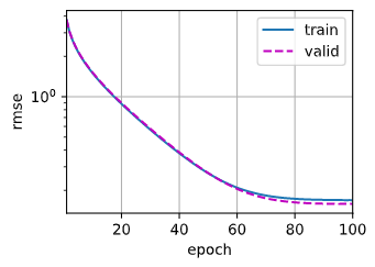
d2l.plot(list(range(1, num_epochs + 1)), [train_ls, valid_ls],
xlabel='epoch', ylabel='rmse', xlim=[1, num_epochs],
legend=['train', 'valid'], yscale='log')
print(f'折{i + 1},训练log rmse{float(train_ls[-1]):f}, '
f'验证log rmse{float(valid_ls[-1]):f}')
return train_l_sum / k, valid_l_sum / k
|
模型选择
1
2
3
4
5
| k, num_epochs, lr, weight_decay, batch_size = 5, 100, 5, 0, 64
train_l, valid_l = k_fold(k, train_features, train_labels, num_epochs, lr,
weight_decay, batch_size)
print(f'{k}-折验证: 平均训练log rmse: {float(train_l):f}, '
f'平均验证log rmse: {float(valid_l):f}')
|
1
2
3
4
5
6
| 折1,训练log rmse0.169009, 验证log rmse0.158280
折2,训练log rmse0.161859, 验证log rmse0.184443
折3,训练log rmse0.163399, 验证log rmse0.167842
折4,训练log rmse0.166751, 验证log rmse0.153802
折5,训练log rmse0.161531, 验证log rmse0.183778
5-折验证: 平均训练log rmse: 0.164510, 平均验证log rmse: 0.169629
|
生成预测结果
1
2
3
4
5
6
7
8
9
10
11
12
13
14
15
16
17
| def train_and_pred(train_features, test_features, train_labels, test_data,
num_epochs, lr, weight_decay, batch_size):
net = get_net()
train_ls, _ = train(net, train_features, train_labels, None, None,
num_epochs, lr, weight_decay, batch_size)
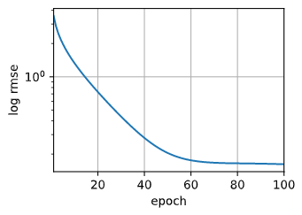
d2l.plot(np.arange(1, num_epochs + 1), [train_ls], xlabel='epoch',
ylabel='log rmse', xlim=[1, num_epochs], yscale='log')
print(f'训练log rmse:{float(train_ls[-1]):f}')
preds = net(test_features).detach().numpy()
test_data['SalePrice'] = pd.Series(preds.reshape(1, -1)[0])
submission = pd.concat([test_data['Id'], test_data['SalePrice']], axis=1)
submission.to_csv('submission.csv', index=False)
train_and_pred(train_features, test_features, train_labels, test_data,
num_epochs, lr, weight_decay, batch_size)
|
将模型应用于测试集,并将生成的预测结果SalePrice按照官方的提交格式保存至submission.csv文件中
可以查看一下该文件:
1
2
3
4
| submission = pd.read_csv('submission.csv')
print(submission.shape)
print(submission)
|
1
2
3
4
5
6
7
8
9
10
11
12
13
14
15
| (1459, 2)
Id SalePrice
0 1461 121965.250
1 1462 163865.200
2 1463 202431.920
3 1464 219286.720
4 1465 178367.160
... ... ...
1454 2915 74494.266
1455 2916 86642.336
1456 2917 213769.400
1457 2918 110917.030
1458 2919 243134.420
[1459 rows x 2 columns]
|
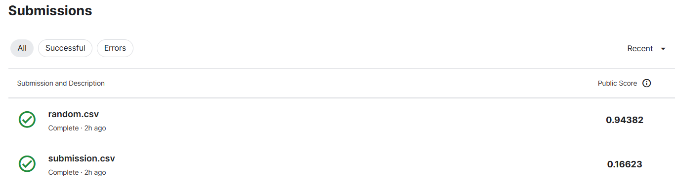
提交结果
在Kaggle上提交结果,排名在2884位。
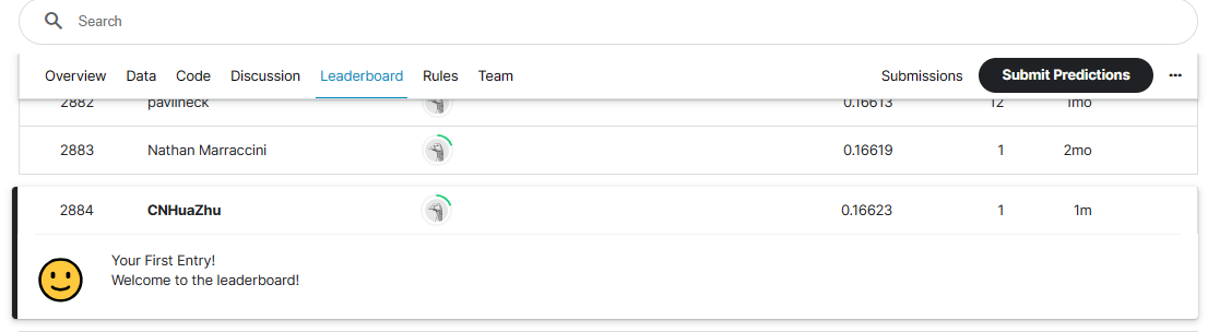
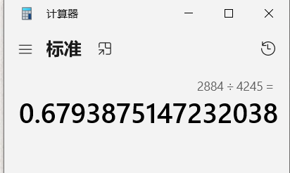
在榜上大概排在68%的位置
后面又按照实际预测值的区间重新随机生成数据,进行提交
1
2
3
4
5
6
7
8
9
10
11
12
13
|
df = pd.read_csv('submission.csv')
max_value = df['SalePrice'].max()
min_value = df['SalePrice'].min()
df['SalePrice'] = np.random.uniform(max_value, min_value, len(df))
df['SalePrice'] = df['SalePrice'].round(3)
df.to_csv('random.csv', index=False)
|
1
2
3
4
| random_file = pd.read_csv('random.csv')
print(random_file.shape)
print(random_file)
|
1
2
3
4
5
6
7
8
9
10
11
12
13
14
15
| (1459, 2)
Id SalePrice
0 1461 497690.627
1 1462 346754.047
2 1463 138443.436
3 1464 586975.087
4 1465 482866.969
... ... ...
1454 2915 534270.138
1455 2916 92022.063
1456 2917 383836.608
1457 2918 593836.710
1458 2919 156347.855
[1459 rows x 2 columns]
|
提交随机预测值查看,结果就要差很多了。
后记
后面可以再修改模型,改动一些超参数,优化检测。
(很经典的一道题目,榜也已经被刷到几乎没有误差了)
 微信
微信 支付宝
支付宝